By Amy Katz, Conservation Director
Photo in header by Brent Calver, courtesy of Nature Conservancy of Canada
This spring, in between house projects and running around in the wildflowers with my girlfriends and my dog, I am integrating a new connectivity model into our Keep It Connected science strategy.
Heart of the Rockies Initiative created the Keep It Connected program to help our member land trusts respond to the growing demand from landowners seeking tools to retain the agricultural, wildlife, and open space values of their land by showcasing private lands that are ready to conserve now and are vital to supporting wildlife connectivity in our region. Since the inception of the program, we have relied on peer-reviewed, service-area wide models to help us determine where the most suitable wildlife connectivity exists.
Over the last several years, we have been using a coarse-scale, species-agnositic, omnidirectional wildlife connectivity model, or, in simpler terms, a model with a large geographic extent and a relatively low resolution that measures general connectivity based on the path of least resistance in every direction, to assess the large-scale wildlife connectivity context of Keep It Connected projects. We consider this model both before we bring these projects to the Heart of the Rockies Foundation board to be approved for the portfolio and also as we are making decisions about which projects to put in front of specific funders.
The model we have been using to date is from a paper exploring how different types of resistance surfaces, or spatial layers representing the varying cost of moving across a geographically diverse landscape, affect identification of suitable connectivity (Belote et al. 2022). There are many ways of defining resistance, or cost, but the most common is through a human modification index (HMI). A HMI quantifies the degree of human modification happening across a landscape, typically including a temporal component, or measuring through time. This particular paper used a HMI that included the following human stressors: urban and built-up, crop and pasture lands, livestock grazing, oil and gas production, mining and quarrying, power generation (renewable and nonrenewable), roads, railways, power lines and towers, logging and wood harvesting, human intrusion, reservoirs, and air pollution (Theobald et al. 2020).
The authors ran their connectivity model three different times, each time assuming a different species tolerance to this HMI to account for the fact that some species are more tolerant of human modification than others. We used the human-tolerant scenario based on the author’s suggestion that the output from this parameter better represented expected and observed animal movement.
The paper also explores how running the model across varying spatial scales affects suitability. For example, running it across 30 kilometers better represents short-range dispersal and small-scale connectivity, while a coarse, 300 kilometer scale will show landscape-level connectivity aimed at managing connectivity across a large region. We chose to use the middle scale of 150 kilometers as it better represented both local and regional connectivity.
The model worked well to contextualize projects on a landscape level but did not scale down well to the individual project level. In addition to this issue of scale, the HMI resistance layer relied solely on human-centric parameters and did not consider any topographical features. This is a reasonable parameter given the assumption that maintaining connectivity through relatively undeveloped, natural lands is favorable for the largest number of species, as the authors call out in the paper. However, over the years, we learned that using a human-centric cost layer such as this HMI often resulted in an overemphasis of north-south corridors that avoid agricultural fields, riparian areas close to roads or powerlines, and working ranches: the very areas we are working to protect.
We have been searching for an alternative model to integrate into our decision making process that better highlights east-west corridors at a finer scale. In early 2026, a research team out of Canada led by Paul O’Brien at the Ontario Ministry of Natural Resources published a paper detailing a new connectivity model we feel will meet these goals.
The paper expands on a Canada-wide model published in 2023, which used an approach similar to that of our current connectivity model but added natural features known to affect terrestrial animal movement, such as elevation and slope, into their cost layer (Pither et al. 2023). Additionally, the authors ran the model at a 300 meter by 300 meter resolution, allowing for significantly finer scalability. The authors found the model to be supported by independent movement data across several species, and a subsequent paper further demonstrated the model’s ability to predict a breadth of species’ movement (Brennan et al. 2025).
The 2026 paper extends the same methods into the United States, ultimately producing a seamless transboundary connectivity map between the two countries (O’Brien et al. 2026). Beyond recreating the model first done in Canada in the U.S., the authors presented three case studies to highlight potential application of transboundary connectivity conservation, including a successful validation of elk connectivity based on GPS locations between Montana, Alberta, and British Columbia.
As we began doing our own validation of the model, we found it was successfully highlighting important east-west corridors and valley bottoms. I reached out to Paul O’Brien to ask him why he thought the model was picking up these corridors so well, and he hypothesized the emphasis on high versus low elevation in the cost surface was likely the reason for this: the current is essentially going around mountain ranges and areas of higher elevation given their higher cost, causing the model to predict high connectivity through relatively undeveloped valley bottoms in between. Not only was the model predicting connectivity well on private lands, but it was also pulling out key pinch points, such as a small area across Highway 93 outside of Darby, Montana in the Bitterroot Valley, where public land extends very close to the road on both sides and therefore sees a high volume of wildlife road crossings (Fig. 1). Paul said these models are often good at identifying pinch points or bottlenecks in situations where low cost areas are near high cost areas, or in this case, where relatively undeveloped private lands are adjacent to roads and topographically complex, difficult to navigate mountain ranges.
We started to have substantial confidence in the model’s ability to highlight generalized connectivity and specific pinch points across our service area, and recently created two new layers, generalized connectivity and key pinch points, from the raw current flow data that land trust members can use to assess potential new Keep It Connected projects (Fig. 2). We are excited to continue hearing from our land trusts about how the model is performing for them as we continue to advance the scientific basis and strategy of the Keep It Connected program.
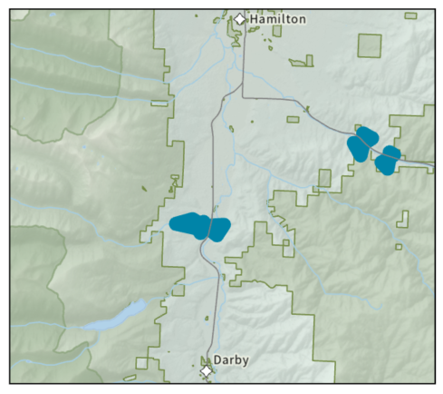
Figure 1. Pinch point shown in blue, created by buffering the top 5% of raw current density values by 500 meters. The pinch point just north of Darby, Montana is in between large swaths of public land that extend particularly close to the highway in that spot.
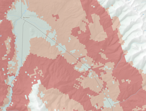
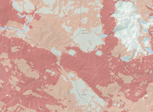
Figure 2. Two examples of east-west connectivity corridors identified by the model south of Salmon, Idaho and north of Missoula, Montana. High connectivity values shown in red and medium connectivity values shown in orange. Keep It Connected has funded projects within many of these high connectivity zones.